Download AFFINImeter ITC Advanced for Windows

We’ve released AFFINImeter ITC Advanced 1.2.0 for Windows

Do you want to install and use AFFINImeter in your computer? Now you can.

Go ahead and download AFFINImeter ITC for Windows right now (only for 64 bits computers).
Upon download, all users will get a FREE 30 days trial version for AFFINImeter ITC Advanced, including: KinITC, ITC and TA data analysis, Model builder, Design complex fitting and simulation projects for ITC, and a new tool: the rawdata experiments simulator.

Users who purchased a license for the web version have the same license for the Windows version. Just contact us at info@affinimeter.com to activate it.


Release notes for 1.2.0 (Update is recommended):

Important updates have been performed in the windows version of the AFFINImeter-ITC software. 

The analysis has implemented the accurate determination of concentrations recently published by Philippe Dumas: (see https://www.biorxiv.org/content/10.1101/512780v1.full).

This update breaks backwards compatibility: this means that all previously created projects (.affprojects) will not be compatible with this version (they will not load in the application or will throw some errors). The previously processed itc/ta raw data should be processed again to update the accurate calculation of concentrations in the equilibrium isotherm.

Other problems/issues fixed:

  • [Fixed] Fitting Projects Output may show incorrect results while performing complex fittings.
  • [Added] Fitting Projects now have an option to download a ZIP file containing all charts in the project, and also some new and specific ones.
  • [Added] Presentation of local minima for fitting projects was improved.
  • [Added/Fixed] Y labels, ticks and names
    • Y values/ticks will have an exponential format instead of the SI prefixes
    • Some Y label names were fixed
  • [Fixed] “Auto” setting in KinITC will stay active after deleting points in the Isotherm, if user the user has it active. Previously, after changing/deleting points in the isotherm, that setting was lost.
  • [Added] Included more references in the Help Section

Analysis of Fluorescence Polarization competition assays with AFFINImeter

Fluorescence Polarization competition assays are widely used in numerous research fields to determine the affinity of unlabeled ligands that compete with a fluorescent probe for binding with the same macromolecule. Herein, we show how to perform a thoughtful analysis of these experiments with AFFINImeter for spectroscopic techniques, to elucidate, not just IC50 values, but also a quantitative direct measurement (KA) of the binding affinity.


Introduction


Fluorescence polarization (FP) is a powerful technique that nowadays is widely utilized in high-throughput screening (HTS) and drug discovery (1). In FP assays monitoring a binding event is possible mainly because this technique is sensitive to changes in molecular weight. The assay requires of a fluorescent molecule (the probe) that is excited by plane-polarized light. For small molecules, the initial polarization decreases rapidly due to rotational diffusion during the lifetime of the fluorescence, which results in low fluorescence polarization. When the small fluorescent molecule binds to a larger molecule (and consequently of slower rotation) an increased fluorescent polarization is observed (Fig. 1).
Advances in experimental aspects of the technique like assay design and fluorescent probes is enabling the application of FP to increasingly complex biological processes (1).

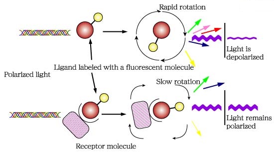
Fig.1. The principle of fluorescence polarization (2).


Frequently, a competition displacement assay format is used in FP experiments where a fluorescent labelled molecule bound to a macromolecule is displaced by an unlabeled molecule with the consequent decrease of polarization. This assay yields a quantitative measure of IC50 values (half maximal inhibitory concentration) of the unlabeled competitors. However, IC50 does not provide a direct measure of affinity and the calculation of the binding constant (KA) is often desirable. In this sense, the software AFFINImeter Spectroscopy offers exclusive analysis tools to perform a thoughtful analysis of FP competition assays, to directly deliver values of binding constants of the interaction between the competitor and the macromolecule. As an illustrative example, we present herein the use of AFFINImeter Spectroscopy for the analysis of FP competition assays to characterize oligosaccharide –protein interactions.


FP competition assays to study the binding between midkine and chondroitin sulfate-like tetrasaccharides


Midkine is a cytokine which biological activity is regulated by its binding with glycosaminoglycans (GAGs), such as heparin and chondroitin sulfate. To better understand these recognition processes Pedro M. Nieto et al. have recently reported the binding of a series of synthetic chondroitin sulfate-like tetrasaccharides with midkine, using FP competition assays (3). First, the direct binding of midkine and a fluorescein labelled heparin hexasaccharide (fluorescent probe) was monitored in a direct FP titration (Fig. 2a). Second, FP competition assays were performed, in which the polarization of samples containing fixed concentrations of midkine and fluorescent probe was recorded in the presence of increasing concentrations of different synthetic sugars to obtain the corresponding IC50 values (Fig. 2b) (3).


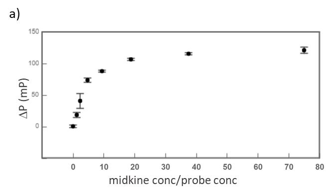
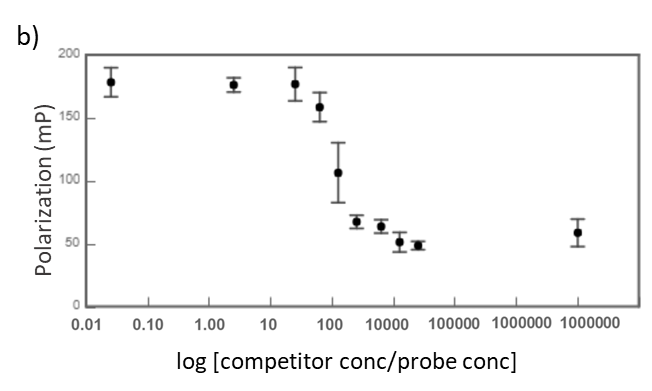
Fig.2. a) Binding curve of the titration of fluorescent probe with midkine 3a;b) Representative competition curve (semi-log plot) of an FP competition assay where the fluorescent probe is displaced from a pre-formed complex with midkine by the competitor.


Analysis of FP competition assays with AFFINImeter Spectroscopy


The determination of KA of the interaction of the unlabeled ligand with the macromolecule in an FP competition assay is possible if the corresponding curve is analyzed using a competitive binding model where two equilibria are described, one between the free species and the macromolecule–probe complex and one between the free species and the macromolecule–competitor complex. In this analysis, the KA value of the interaction between probe and macromolecule can be fixed (as it can be previously calculated from the direct binding experiment) in order to determine KA of the competitor-macromolecule complex. Yet, a more robust approach consists of a global analysis of direct and competitive curves where constraints between experimental parameters are imposed. Using this approach, we have used AFFINImeter Spectroscopy in the analysis of data from the direct measurement of the fluorescent labelled hexasaccharide binding to midkine and together with data from the displacement assay using an unlabeled, synthetic disaccharide as a competitor (4).

An AFFINImeter fitting project was generated where the curve from the direct titration and two curves from replicates of the competitive assay were included. A 1:1 simple binding model and a competitive model were used to fit direct and competitive data, respectively (Fig. 3).

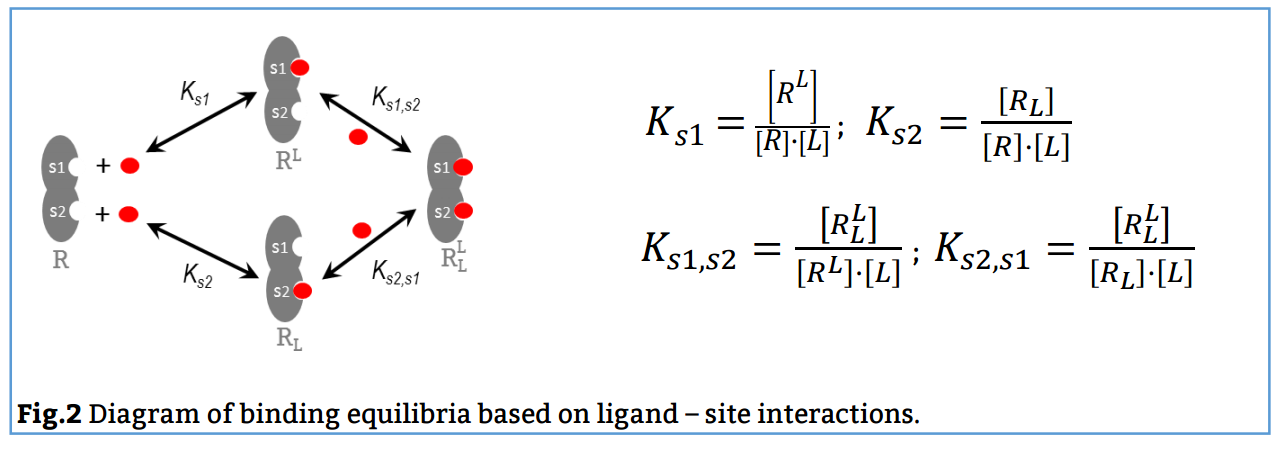
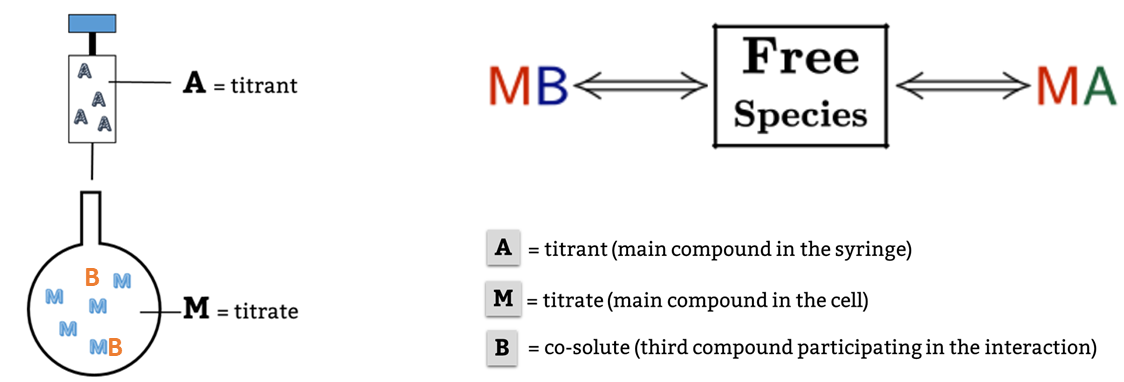
Fig.3. Schematic representation of the binding models used to fit the FP data.5 These models can be easily built with the “model builder” tool of AFFINImeter where a) in the 1:1 model “M” represents the species sensitive to binding (fluorescent probe) and “A” represents the titrant (midkine); b) in the competitive model “M” is the sensitive species (probe), A is the titrant (competitor) and B is a third species involved in the event (midkine in a preformed complex with the probe).


In the analysis, the fitting parameters considered were the KA of each complex, the signal value of the unbound state (s0), and the maximum signal change (Δsmax) of the midkine-probe complex formation. Δsmax of the midkine-competitor complex is equal to zero because the competitor is not fluorescent. Since midkine-probe binding is present in both models, restrictions were made considering that KA and Δsmax of the 1:1 model (FS↔MA) are equal to the same parameters describing this equilibrium in the competitive model (FS↔MB). Besides, s0 was common between replicates of the competitive assay. It is worth to mention that the curves analyzed are the mean of three replicate experiments and the corresponding standard deviation of the curve data points are also considered in the fitting process.  The global analysis performed in this way returned the KA of the interaction of midkine with the probe, (3.09 ± 0.18)*107 M-1, and with the competitor, (5.30 ± 0.52)*106 M-1 (Fig. 4). Additionally, AFFINImeter automatically generates the species distribution plot, valuable in the interpretation of results. The species distribution plot of Fig. 4c shows the displacement of the probe by the unlabeled disaccharide in the competition assay.


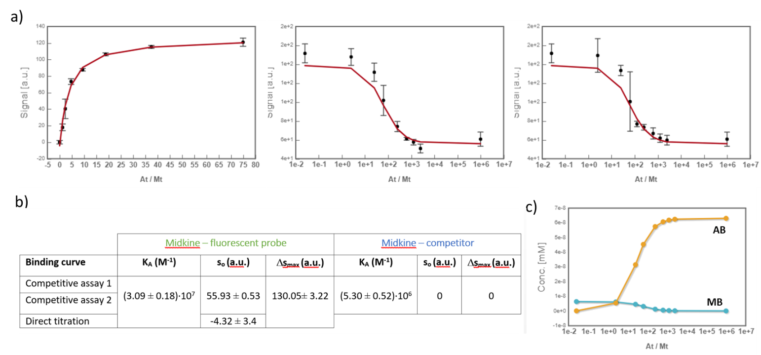
Fig.4. a) Global analysis of FP curves from the direct titration of probe (10 nM) with midkine (12 – 750 nM) and from a competitive assay consisting of a sample with probe (10 nM) and midkine (63 nM) where the competitor is added at increasing concentrations (0 – 20 mM). Curves from two replicates of the competitive assay were used in the analysis. All the polarization values are the average of three replicate wells and the error bars represent the corresponding standard deviation; b) values of KA, s0 and Δsmax determined for each equilibrium; c) species distribution semi-log plot of the competitive assay.


Conclusions


This case study exemplifies the utility of AFFINImeter Spectroscopy in the analysis of FP competitive binding assays. The advantages of using this software rely on the possibility to obtain reliable KA values of the binding between competitor and macromolecule from a global analysis where KA and Δsmax of the probe-macromolecule complex, are shared parameters between curves (they are not pre-determined fixed parameters). Besides, standard deviation between replicates is taken into account in the fitting process. Ultimately, these tools provide a more robust analysis and reliable characterization of binding interactions monitored through competitive assays.


Try AFFINImeter Spectroscopy

Acknowledgements


We would like to thank Dr Pedro Nieto Mesa and Dr José Luis de Paz Carrera from the Institute of Chemical Research (IIQ) of the Spanish National Research Council (CSIC), for kindly share with us the FP data presented herein.


References & Notes


1 Hall, M.; Yasgar, A.; Peryea, T.; Braisted, J.; Jadhav, A.; Simeonov, A.; Coussens, N. Fluorescence Polarization Assays In High-Throughput Screening And Drug Discovery: A Review. Methods and Applications in Fluorescence 2016, 4, 022001.

2 This figure has been taken from http://glycoforum.gr.jp/science/word/glycotechnology/GT-C06E.html.

3 a) Solera, C.; Macchione, G.; Maza, S.; Kayser, M.; Corzana, F.; de Paz, J.; Nieto, P. Chondroitin Sulfate Tetrasaccharides: Synthesis, Three-Dimensional Structure And Interaction With Midkine. Chemistry – A European Journal 2016, 22, 2356-2369; b) Maza, S.; Gandia-Aguado, N.; de Paz, J.; Nieto, P. Fluorous-Tag Assisted Synthesis Of A Glycosaminoglycan Mimetic Tetrasaccharide As A High-Affinity FGF-2 And Midkine Ligand. Bioorganic & Medicinal Chemistry 2018, 26, 1076-1085.

4 The competitor is a synthetic disulfated disaccharide described in ref. 3b as compound 18.

5 These model were created with the “model builder” tool, exclusive of AFFINImeter. For more information go to AFFINImeter knowledge center.

What does it look like to you?

It might look like a plain hat or an elephant being eaten by a boa constrictor, but actually, the shape of this curve looks like a typical spectrum of UV-Vis determined by changes in the intensity of this energy and also it represents the logo of our new software:

AFFINImeter for spectroscopic techniques!


Hence, we want to take this opportunity to launch AFFINImeter Spectroscopy software.

It is a new software for the processing and advanced analysis of binding isotherms obtained from different spectroscopic techniques: 1D-NMR, Uv-vis, fluorescence, circular dichroism, differential scanning fluorimetry…


…and from now on, you will be able to start using it:

Get a free trial


To get started, we have prepared some scientific material as an example of how to use AFFINImeter Spectroscopy:


We have prepared a special offer to celebrate the launch of AFFINImeter for Spectroscopic techniques.
Using this code coupon you will get a 25% off*, to buy through our online shop:

Spectroscopy_coupon


 You can also ask for a quotation here 
 
 
*The discount will be applied until 2018/03/03.

Global fitting: the key for a robust analysis

Download use case: Global Fitting


The Indian parable of “The six blind men and the elephant” tells the story of six blind men who touch an elephant in the hope of learning what it is like. As each one can only feel a different part of the animal the individual conclusions obtained are in disagreement and none of them provides a real view of the full elephant. “only by sharing what each of you knows can you possibly reach a true understanding”; that´s the moral behind this nice story.


Fig 1: The six blind men and the elephant: only a global analysis of the overall data provides a true understanding.

The binding assay(s) achieved to characterize a molecular interaction often provides not just one, but several binding curves from which the affinity constant is obtained.
Sometimes, an individual fit of these curves yield a set of binding constants that are significantly different from them; this result can be very confusing because, in principle, these binding curves are a representation of the same binding event and should converge to provide the analogous information. Often, the explanation for this behaviour is that the different curves indeed provide only partial and/or different information of the interaction, not enough to unequivocally determine the binding affinity through individual analysis.


“It´s like feeling only a separate part of the elephant”


This is a typical scenario when facing the study of complex binding events that involve more than one equilibrium and several binding curves are obtained, i.e. from different frequencies of the spectra in a titration experiment, from data registered using different techniques (ITC, NMR, Optical Spectroscopies…) and/or from experiments performed at different concentrations of the species participating in the binding event.


Analogous to the parable of the six men and the elephant, the way to get a true understanding of the binding event consist of the global analysis of the different curves.

Fig 2: The binding curve obtained from 2D NMR titrations.


Being aware of the relevance of global analysis, in AFFINImeter we count with the possibility to perform Global fitting of multiple data to tailored binding models where one or more fitting parameters are shared between isotherms. The number and identity of the parameters shared are selected by the user.
Moreover, two or more parameters can be related through mathematical relationships designed by the user. All these features make our global fitting tool the most potent among others to perform a robust analysis of binding data of complex interactions.

About the disuses of  Isothermal Titration Calorimetry in drug discovery research

Isothermal Titration Calorimetry (ITC) is the gold standard for the calculation of affinity in molecular interactions. Many times, researchers claim that the high consumption of sample does not offset the use of ITC for Kd calculation.
Conversely, ITC hides many surprises in the acquisition data that can provide more information in a single experiment that other techniques that are more expensive and more complicated to use.

Download the PDF file of Implementation of kinITC into AFFINImeter


1. ITC collects data from the interaction as a function of time that can be analyzed to obtain kinetic information (kon and koff values). It can cover a very similar range as Surface Plasmon Resonance in a “label-free” and “in-solution” manner (Fig 1).

2. ITC can also provide valuable information about the mechanism of interaction. The high sensitivity of the ITC sensor makes it sensitive to more intriguing interactions as conformational changes, cooperativity…

Using a global fitting approach for the analysis of the isotherms and a model builder to create tailored binding models, the different mechanisms of interaction can be confirmed and characterized.

Find attached a couple of publications describing the application of this new method for ITC data analysis:

Download the PDF file of Implementation of kinITC into AFFINImeter


The concepts of stoichiometric and site binding constants

Download: The concepts of stoichiometric and site binding constants

The interaction between a monovalent ligand L and a multivalent receptor R involves the presence of various species, including the complex of R fully saturated with a number of ligands, and intermediate complexes of R partially saturated. This scenario can be described in terms of reaction schemes following two approaches:


  1. Based on equilibria between existing stoichiometric species (Stoichiometric approach).
  2. Based on equilibria between L and specific interaction sites of R (independent sites approach).
For a better understanding, let´s consider a particular case where L binds to a bivalent receptor:

1. Stoichiometric approach

This approach uses reaction schemes based on equilibria between stoichiometric species and yields stoichiometric binding constants. A model based on stoichiometric equilibria is valid to fit data of both independent and non-independent events and therefore, it is of wider applicability.

Here, the reaction scheme includes a first equilibrium between the free species and the intermediate RL and the second equilibrium between RL + L and RL2 (Fig. 1). The corresponding binding constants, K1 and K2, are denominated stoichiometric binding constants since they refer to equilibria between stoichiometric species.


2. Independent site approach

This approach uses a reaction scheme based on the binding of the ligand to individual sites present in the receptor and considering that all the sites are independent; thus, it supplies site binding constants.

In this case, the reaction scheme considers the presence of two sites in the bivalent receptor and two intermediate complexes (R, L and RL) formed when the ligand binds to s1 or s2 and consequently, the existence of a total of 4 equilibria (Fig. 2). The corresponding binding constants, Ks1, Ks2, Ks1s2 and Ks2s1, are denominated site binding constants since they refer to equilibria between L each specific site of R.


If you want to know more about how to get the stoichiometry (number of sites) and site binding constants with the independent sites approach you can click on the following button:


AFFINImeter binding models for Nuclear Magnetic Resonance

AFFINImeter is already well known in ITC binding data analysis for providing the possibility to use tailored binding models created by the user. The models are generated with the tool “model builder” that includes a letter code “M-A-B” to describe titrate (M), titrant (A) and if necessary, the presence of a third species (B) (Figure 1).


Fig.1 Example of a competitive binding model created in AFFINImeter where the titrant in syringe “A” binds to the titrate in cell “M” to form a 1:1 complex “MA” and a second ligand “B” mixed in the cell with “M” forms the complex “MB” and thus competes with “A”.


Following the same approach, the binding models available for the software AFFINImeter for Nuclear Magnetic Resonance are generated with the model builder and based on the “MAB” code. But there are significant differences between ITC and NMR data analysis when the time comes to select a binding model from AFFINImeter, which have an origin in the inherent characteristics of each technique and in the different experimental design. In chemical shift perturbation (CSP) NMR titration experiments, the observed parameter used to monitor the progress of the binding event is the chemical shift of titrate resonance signals. Hence, the models used for NMR data analysis require the presence of compound “M” (titrate) as it is the species from which changes associated with the binding process are monitored. Conversely, in ITC the observed parameter is the heat change upon interaction and this parameter is not necessarily linked to a particular species “M”, “A” or “B”.

An illustrative example is the evaluation of a monomer-dimer self-association process using NMR or ITC. In NMR, the standard experimental setup would consist in the incremental dilution of the compound sample at high concentration in the NMR tube, to monitor dimer dissociation (Figure 2a). In ITC the standard experimental setup would consist in a titration of the compound sample at high concentration in the syringe (species “A” according to the AFFINImeter code) into the calorimetric cell filled up with solvent (Figure 2b).


Fig.2 Representation of experimental setup for a) NMR dilution experiment and b) ITC dilution experiments. The corresponding schemes of AFFINImeter binding models for data analysis are shown.


Would you like to know more about AFFINImeter for Nuclear Magnetic Resonance? Press the button below:

AFFINImeter-NMR


MicroCal User´s day in Madrid

The next April 19th will be taking place in Madrid the MicroCal user´s day. The event will be held at the Institute of Chemical Physics Rocasolano.

The basics and applications of the ITC -Isothermal titration Calorimetry and DSC -Differential scanning calorimetry technologies will be treated. It will be an excellent event with very interesting talks and nice place for catch up of these applications.

We are pleased to announce that Dr Juan Sabín (Co-founder & Product Designer) will be giving a presentation about AFFINImeter, the software for Isothermal Titration Calorimetry data analysis.

Additionally, Dr Raúl Pacheco application specialist from Malvern Instruments, Dr Margarita Menendez from the Institute of Chemical Physics Rocasolano and Dr Javier Murciano from the University of Granada will also attend the event.

The Microcal user´s day has been organised by Malvern Instruments, CSIC-Spanish National Research Council, Institute of Chemical Physics Rocasolano and Iesmat.

For more information:

Microcal user´s day Madrid.

5 Tips to optimize your ITC experiments for kinetic analysis.

Since the method KinITC was implemented in AFFINImeter many researchers have been using it to obtain kinetic information of binding interactions from ITC data; the good news is that no special experimental setup different from the standard ITC experiment is required to register data for kinetic analysis! The information is derived from analysis of the thermogram of regular ITC titrations and therefore one can obtain kinetic information from old ITC data right away.

There are few recommendations though if you are planning to perform new ITC experiments, focused on getting high-quality data for kinetic analysis:

1) Set the time between successive power measurements to 1s or 2s. This will give a better definition of the thermogram peaks and therefore a more precise calculation of the equilibration times.

2) Set the time recording the baseline before the first injection to 1 or 2 minutes. In order to have a good reference when determining the signal baseline.

3) Leave enough time between injections so that a full equilibration for the overall set of injections is registered.

4) Clean thoroughly the instrument before the experiment. This is fundamental to optimize the response time of the instrument, which strongly determines the sensitivity of the kinetic analysis.

5) A high gain feedback mode is recommended in order provide the fastest response time (but, be careful because a high feedback mode can also generate signal overshooting after injection, which greatly difficulties the kinetic analysis! If overshooting happens, don´t use high gain model).

Need more information about this subject? Contact the Scientific team of AFFINImeter at info@affinimeter.com.

Follow these simple tips to increase the quality of your ITC data for kinetic analysis

Figure Junio2016

KinITC for TA and MicroCal Calorimeters – New version Release!

During the last months we’ve contacted you asking your opinion and experience with the software. Thanks to all your suggestions and comments we have improved the previous version of the software to make it easier, faster and more versatile.

What’s new in AFFINImeter?

  • Availability of KinITC for TA and Microcal data files.
  • Inclusion of Multi Temperature Analysis: Van’t Hoff and Eyring plots
  • The project management section has improved, now you can easily organize your projects in Folders/Subfolders and move them from one to another.


Easier, Faster and more Versatile!

In this new version you will find several changes adressed to improve the user experience of the software, adding more features, making it easier and faster to user, and more versatile.


Go to the software!