A few days ago AFFINImeter launched an Isothermal Titration Calorimetry (ITC) data analysis challenge. Here the participant had to globally analyse a set of Isothermal Titration Calorimetry experiments using AFFINImeter and get the thermodynamic and structural parameters of the interaction between both molecules (the receptor protein and the ligand).
The participants in this contest had the opportunity to demonstrate their ability to propose the right model for a given binding isotherm as well as to get the corresponding parameters upon fitting using AFFINImeter. On their side, less experienced participants had the opportunity to:
- Learn the difference between stoichiometric and site equilibrium constants.
- Perform a global analysis of Isothermal Titration calorimetry data
- How to find the, eventually unknown, concentration of active protein in a given experiment
During the last days we though it might be useful to help you throughout the fittings proposed for the contest. Therefore, we have prepared a video that explains, step by step, How to fit CURVE 1. IMPORTANTLY, this information will be of great help to solve step 2, the global fitting of CURVES 1-4.
The data proposed for the contest will remain available here, in case you want to learn more about it or to try it by yourself.
Tips to solve Step 1
Tips to solve Step 2
Here are some tips to solve step 2 (global fitting of curves 1-4):
When talking about linking parameters think of the thermodynamic parameters (K and DH) that are common among curves. In other words, determine which curves describe the same binding event(s):
Dr. Brooks gave us a set of four curves:
CURVE 1 and CURVE 2 describe the interaction of L1 and L2 with the protein, respectively. They describe different interaction events and therefore they don´t have any thermodynamic parameter in common.
CURVE 3 corresponds to a competitive experiment of a mixture of L1 and L2 binding to the protein. This means that, it has the thermodynamic information of both interaction events: CURVE 3 will share thermodynamic parameters with CURVE 1 and CURVE 2…(and also CURVE 4).
CURVE 4 is also a competitive experiment, similar to CURVE 3 and again, has the thermodynamic information of both interactions. Then, CURVE 4 shares thermodynamic parameters with CURVE 1, CURVE 2 and CURVE 3.
Have a look at the following drawing, with a summary of the parameters that are common among Dr. Brooks curves:

NOW,…how do we define all this information into our AFFINImeter global fitting? We have to “link” parameters among curves to “tell” AFFINImeter that we are considering those parameters as equal.
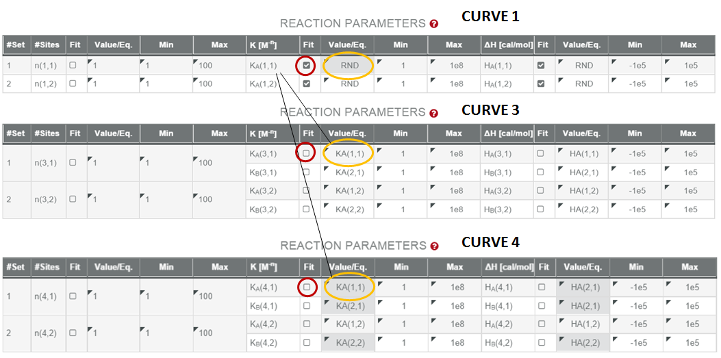
As an example, here are the steps to follow in order to link the parameter in CURVES 1, 3 and 4 that correspond to the association constant of L1 binding to s1 of the protein:
1. Click on the button “link parameters” and then click on the Value/eq box corresponding to the parameter K of CURVE 1 that describes the association constant of L1 to s1.
2. Click on the Value/eq box corresponding to the parameter of CURVE 3 that defines the association constant of L1 to s1.
3. Click on the Value/eq box corresponding to the parameter of CURVE 4 that defines the association constant of L1 to s1.
4. Click on the button “Done” to finish and leave the link parameter mode (NOTE: when you are in the link parameter mode all the functions in the screen are locked except the link function. In order to recover all the functionalities you have to click on “Done”).
5. IMPORTANTLY! The box “FIT” has to be checked for the parameter K of CURVE 1 but it has to be unchecked for the parameter K of CURVES 3 and 4, since now they are related to K of CURVE 1.
Here is a picture that shows how the settings of my project look like after the steps described above: