Global fitting: the key for a robust analysis

Download use case: Global Fitting


The Indian parable of “The six blind men and the elephant” tells the story of six blind men who touch an elephant in the hope of learning what it is like. As each one can only feel a different part of the animal the individual conclusions obtained are in disagreement and none of them provides a real view of the full elephant. “only by sharing what each of you knows can you possibly reach a true understanding”; that´s the moral behind this nice story.


Fig 1: The six blind men and the elephant: only a global analysis of the overall data provides a true understanding.

The binding assay(s) achieved to characterize a molecular interaction often provides not just one, but several binding curves from which the affinity constant is obtained.
Sometimes, an individual fit of these curves yield a set of binding constants that are significantly different from them; this result can be very confusing because, in principle, these binding curves are a representation of the same binding event and should converge to provide the analogous information. Often, the explanation for this behaviour is that the different curves indeed provide only partial and/or different information of the interaction, not enough to unequivocally determine the binding affinity through individual analysis.


“It´s like feeling only a separate part of the elephant”


This is a typical scenario when facing the study of complex binding events that involve more than one equilibrium and several binding curves are obtained, i.e. from different frequencies of the spectra in a titration experiment, from data registered using different techniques (ITC, NMR, Optical Spectroscopies…) and/or from experiments performed at different concentrations of the species participating in the binding event.


Analogous to the parable of the six men and the elephant, the way to get a true understanding of the binding event consist of the global analysis of the different curves.

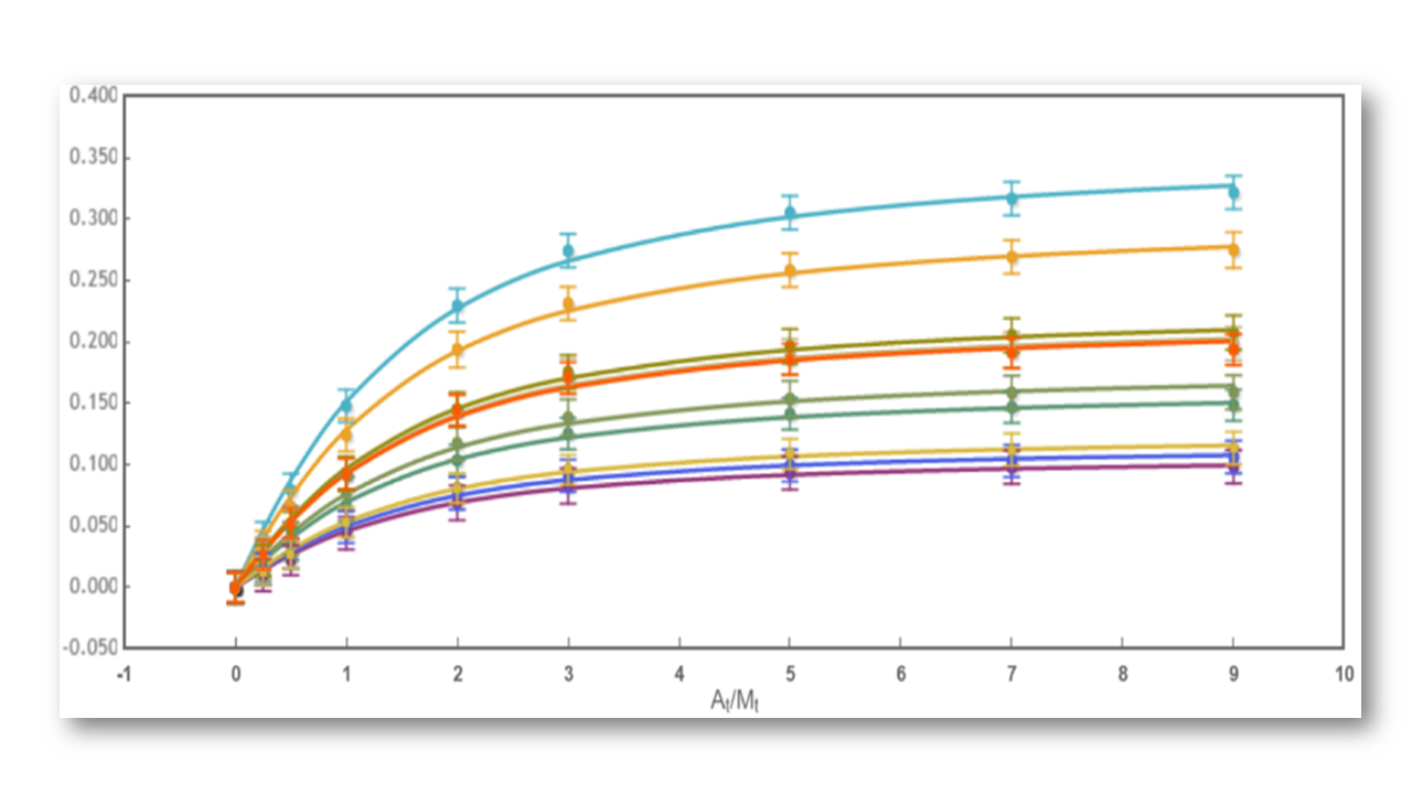
Fig 2: The binding curve obtained from 2D NMR titrations.


Being aware of the relevance of global analysis, in AFFINImeter we count with the possibility to perform Global fitting of multiple data to tailored binding models where one or more fitting parameters are shared between isotherms. The number and identity of the parameters shared are selected by the user.
Moreover, two or more parameters can be related through mathematical relationships designed by the user. All these features make our global fitting tool the most potent among others to perform a robust analysis of binding data of complex interactions.

AFFINImeter binding models for Nuclear Magnetic Resonance

AFFINImeter is already well known in ITC binding data analysis for providing the possibility to use tailored binding models created by the user. The models are generated with the tool “model builder” that includes a letter code “M-A-B” to describe titrate (M), titrant (A) and if necessary, the presence of a third species (B) (Figure 1).


Fig.1 Example of a competitive binding model created in AFFINImeter where the titrant in syringe “A” binds to the titrate in cell “M” to form a 1:1 complex “MA” and a second ligand “B” mixed in the cell with “M” forms the complex “MB” and thus competes with “A”.


Following the same approach, the binding models available for the software AFFINImeter for Nuclear Magnetic Resonance are generated with the model builder and based on the “MAB” code. But there are significant differences between ITC and NMR data analysis when the time comes to select a binding model from AFFINImeter, which have an origin in the inherent characteristics of each technique and in the different experimental design. In chemical shift perturbation (CSP) NMR titration experiments, the observed parameter used to monitor the progress of the binding event is the chemical shift of titrate resonance signals. Hence, the models used for NMR data analysis require the presence of compound “M” (titrate) as it is the species from which changes associated with the binding process are monitored. Conversely, in ITC the observed parameter is the heat change upon interaction and this parameter is not necessarily linked to a particular species “M”, “A” or “B”.

An illustrative example is the evaluation of a monomer-dimer self-association process using NMR or ITC. In NMR, the standard experimental setup would consist in the incremental dilution of the compound sample at high concentration in the NMR tube, to monitor dimer dissociation (Figure 2a). In ITC the standard experimental setup would consist in a titration of the compound sample at high concentration in the syringe (species “A” according to the AFFINImeter code) into the calorimetric cell filled up with solvent (Figure 2b).


Fig.2 Representation of experimental setup for a) NMR dilution experiment and b) ITC dilution experiments. The corresponding schemes of AFFINImeter binding models for data analysis are shown.


Would you like to know more about AFFINImeter for Nuclear Magnetic Resonance? Press the button below:

AFFINImeter-NMR